

Supercharge Your Machine Learning Model Architecture with 1x1 Convolutions
Supercharge Your Machine Learning Model Architecture with 1x1 Convolutions
Learn what 1x1 convs are and how to build lightweight and performant CNNs

Get a list of personally curated and freely accessible ML, NLP, and computer vision resources for FREE on newsletter sign-up.
1x1 convolutions are a powerful tool when designing convolutional neural network (CNN) architectures for your task. We'll go over what 1x1 convolutions are, how they work, and why you should consider using them in your next project.
To read more on this topic see the references section at the bottom. Consider sharing this post with someone who wants to study machine learning.

What do 1x1 convolutions help you achieve?
By incorporating 1x1 convolutions into your CNN architecture, you can achieve:
Reduced model size: Smaller models require less memory with faster training and inference.
Improved efficiency: Less computation is needed for processing data.
Deeper models: The parameter budget that you saved can be reallocated to build deeper, more performant models [3].

Convolution filtered in deep learning. [6]

Are you looking to understand convolutions in deep learning better? Check out this excellent visual guide to convolutions [6].
What are 1x1 convolutions?
1x1 convolutions offer a powerful way to improve CNN efficiency. Instead of detecting spatial features, it combines information across channels in the input feature volume.
1x1 convolutions are siblings of the pooling layer. Let’s see where they differ and where they are similar.
A 2x2 max pool aggregates across the spatial dimensions H and W. It would take an input feature from (N, C, H, W) to (N, C, H/2, W/2).
A 1x1 convolution aggregates across the channel dimension C. It can take an input feature from (N, C, H, W) to (N, C’, H, W)1. It is a channel-wise weighted pooling, learning relationships across the channel dimensions of the feature volume.
Visualizing 1x1 convolutions
We have 5x5 spatial locations and 6 channels in the input feature volume. The 1x1 convolution has a filter with 6 channels to match the 6 channels in the input. It has a 1x1 spatial dimension meaning.

The output volume at (x, y) takes the value of the dot product of all channels at (x, y) in the input and the convolution filter. Repeat this for all spatial locations to get the complete output feature map with 1 channel with 5x5 spatial dimensions. Note how both the input and the output maintain the spatial resolution of 5x5 but the channels change from 6 to 1.

Reducing Parameters and Boosting Efficiency
One of the biggest advantages of 1x1 convolutions is their ability to reduce the number of parameters in your model. Here's how:
Traditional convolutions with large filters require numerous parameters.
1x1 convolutions act as a bottleneck, reducing the number of channels before feeding them into computationally expensive operations like larger convolutions with 5x5 and 7x7 filters2.
This translates to a model with a smaller memory footprint and faster training and inference times. This makes it a perfect use case for models meant to run on edge and mobile devices.
Achieving parameter efficiency with 1x1 convolutions: A Numerical Example
Modern neural network architectures consist of multiple repeated blocks of computation. Consider a block that takes a 100 x 20 x 20 feature volume as input and outputs a 40 x 20 x 20 feature volume. Here are 2 possible variants to achieve this.

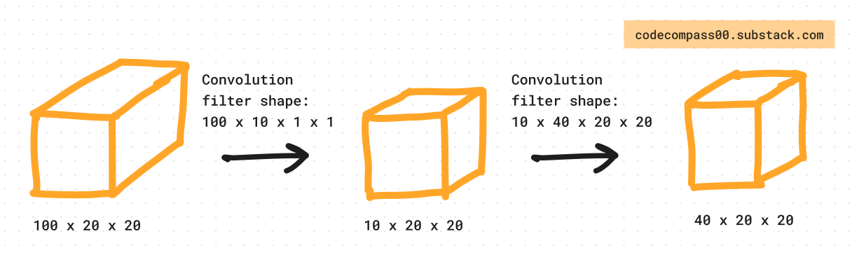
Which of the 2 variants has more parameters?
At a glance, one might conclude that variant #2 has more layers so it likely also has more parameters. Let’s do some quick math to compute the number of parameters used in each variant.
Variant #1: 100 x 40 x 20 x 20 = 1,600,000
Variant #2: 100 x 10 x 1 x 1 + 10 x 40 x 20 x 20 = 161,000
Variant #2 has ~10x less parameters than variant #1. It sounds counterintuitive at first. The 1x1 convolution reduces the channels (dimensionality reduction) making it cheaper to perform the following convolution operation.
When to use 1x1 convolutions?
Before expensive operations: Use them before large convolutions (ideally, use multiple 3x3 convolutions instead of larger filters) to reduce the number of channels processed.
Bottleneck layers: Employ them as bottlenecks in deeper architectures to control model size and complexity.
Famous model architectures using 1x1 convolutions
Inception [1]: Google's Inception models rely heavily on 1x1 convolutions for efficiency and performance gains.
SqueezeNet [5]: SqueezeNet utilizes 1x1 convolutions within its fire modules. This approach significantly reduces the computational cost of the network.
“Replace 3x3 filters with 1x1 filters. Given a budget of a certain number of convolution filters, we will choose to make the majority of these filters 1x1, since a 1x1 filter has 9X fewer parameters than a 3x3 filter.”
ResNet [3]: A widely used architecture, ResNet employs 1x1 convolutions within residual blocks. These filters serve two purposes: introducing non-linearities and controlling the number of channels.
MobileNet [4]: Designed specifically for mobile applications, MobileNet heavily relies on 1x1 convolutions to achieve lightweight and efficient models.
Ready to experiment with 1x1 convolutions? They're a valuable tool to add to your CNN skillset, enabling you to create more efficient and powerful models.
Consider subscribing to get it straight into your mailbox:
Continue reading more:


References
[1] Going Deeper with Convolutions: https://arxiv.org/abs/1409.4842
[2] Network in Network: https://arxiv.org/abs/1312.4400
[3] Deep Residual Learning for Image Recognition: https://arxiv.org/abs/1512.03385
[4] MobileNets: Efficient Convolutional Neural Networks for Mobile Vision Applications: https://arxiv.org/abs/1704.04861
[5] SqueezeNet: AlexNet-level accuracy with 50x fewer parameters and <0.5MB model size: https://arxiv.org/abs/1602.07360
[6] Convolution arithmetic: https://github.com/vdumoulin/conv_arithmetic
Consider sharing this newsletter with somebody who wants to learn about machine learning:
When C’ < C the 1x1 convolution reduces dimensionality.
Ideally, 7x7 and even 5x5 convolutions should be avoided due to their large number of parameters. It has become common practice to replace a bigger convolution with multiple cheaper and smaller convolutions. A 5x5 convolution can be replaced by two 3x3 convolutions. Seemingly counterintuitive, it is more parameter efficient as it reduces parameters from 25 to 18 (for a single filter without bias units).