

Linear Recurrent Units and attention
Linear Recurrent Units and attention
RNNs strike back

I was struck by the recent paper, “Resurrecting Recurrent Neural Networks for Long Sequences” by Orvieto et al.
Especially important observations:
LRU is a special linear type RNN, that can be efficiently parallelized => training is much faster than purely sequential RNNs, and on par with Transformers etc.
Since the RNN can be explicitly unrolled i.e. exactly solved, vanishing or exploding gradients are not an issue since the unrolled solution can be simply parametrized to avoid bad gradients
Inference is fast and efficient, since it’s an RNN, i.e. no need to always feed in long sequences at once but instead just update by feeding in current token
Scales as O(L) in the sequence length L, instead of O(L^2) as with Transformers
No need for weird state space model initializations and whatnot
Probably the most important observation is that linear, diagonal RNNs is all you need (thankfully they didn’t name the paper “All you need is…”)! Check out the details in Appendix E!
Also notable (maybe even more notable) is the predecessor paper by Gupta et al., “Simplifying and Understanding State Space Models with Diagonal Linear RNNs“, which is basically same model but without the initialization etc. tricks.
However, there’s really no kind of attention in the model, which means that this kind of an RNN is probably not going to be as powerful as a Transformer in Natural Language tasks.
I noticed the LRU can be generalized pretty easily to incorporate a “self-attention” term. Here’s the details:
Define the RNN as
with shapes
The $\nu$ and $\theta$ (sorry bout the LaTeX… damn substack can’t compile inline LaTeX) vectors are the same as in the LRU paper. For U = 0 this model is the LRU.
This RNN can also be solved exactly/ unrolled:
(I'm dropping the $\odot$ symbol for elementwise prods from now on and assuming all vector-vector prods are elementwise) where
Let's look at the initial state h_0 independent source term more closely. For the LRU we have U=0 and we get
So we see there's no attention of any kind, just the modulation of the $x_{t-1-s}$ by powers of the complex number $e^{\nu + i \theta}$.
On the other hand, with U != 0, we get
which is a form of self-attention in the sense that there is now a non-local dependence between the inputs at different times.
In addition, this layer is naturally time translation equivariant (because the RNN equation is time translation invariant).
One more interesting difference to Transformers which both these works have neglected is the fact that even if one uses backprop truncated in time (BPTT), the previous state h_0 is an input, which contains information about the inputs before t=0! Transformers don’t carry a “state” like this so every input into a Transformer typically needs to be very long. One interesting experiment would be to try to train a model with sequential batches (instead of typical random access or a shuffled dataset), and either keeping the state h_0 or resetting it to zero.
RWKV
There’s an interesting related project called RWKV by BlinkDL, where the idea is to basically make a recurrent self-attention layer. Here’s the unrolled recurrence (i stands for time i.e. position in the sequence):
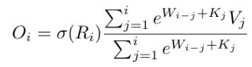
It’s interesting to note that the numerator is like the generalized LRU above, and the denominator is same but with the input Wx replaced with 1! So the RWKV is pretty closely related to linear RNN layers. One thing that’s missing though is the initial state h_0. I think it could be important to keep it, at least when iterating over the dataset in a sequential manner, since it contains information about the previous context, which can definitely be useful when learning about the current (and next) context. I was told in a private communication that the denominator is very important for good performance!
EDIT: oops of course it’s pretty clear why that kind of a normalization by dividing by a similar term is useful - suppose the input sequence x is just white noise, then the cumulative sum over the x will increase as the square root of t! So one nice way to make the series O_i stationary is to use the denominator. Quite clever actually!
Benchmark code
I decided to try out these RNN layers, so here's a pytorch implementation for both sequential and parallel/unrolled case:
EDIT: oops, the sequential code could be optimized a lot by doing the `xs` dependent matrix prods before the loop…
def forward_sequential(h, xs, U, W, nu, theta):
    """Forward pass through the network sequentially over input `xs` of any length.
    NOTE: has no batch dimension. To be batched with `vmap`.

    Args:
        h (torch.tensor): shape [D_h, ]; previous state
        xs (torch.tensor): shape [T, D_x]; input sequence
        U (torch.tensor): Parameter matrix of shape [D_h, D_x]
        W (torch.tensor): Parameter matrix of shape [D_h, D_x]
        xi (torch.tensor): Parameter vector of shape [D_h, ]
        eta (torch.tensor): Parameter vector of shape [D_h, ]
    Returns:
        hs (torch.tensor): shape [T, D_h]; output sequence
    """
    T = xs.shape[0]
    D_h = h.shape[0]
    hs = torch.zeros(T, D_h, device=xs.device)
    for t in range(T):
        h = torch.exp(U @ xs[t] - nu - theta * 1j) * h + W @ xs[t]
        hs[t] = h
    return hs.real


def forward_parallel(h, xs, U, W, nu, theta):
    """Forward pass through the network in parallel over input `xs` of any length by using
    the exact solution of the recurrence relation.
    NOTE: has no batch dimension. To be batched with `vmap`.

    Args:
        h (torch.tensor): shape [D_h, ]; previous state
        xs (torch.tensor): shape [T, D_x]; input sequence
        U (torch.tensor): Parameter matrix of shape [D_h, D_x]
        W (torch.tensor): Parameter matrix of shape [D_h, D_x]
        xi (torch.tensor): Parameter vector of shape [D_h, ]
        eta (torch.tensor): Parameter vector of shape [D_h, ]
    Returns:
        hs (torch.tensor): shape [T, D_h]; output sequence
    """
    gammas = torch.cumsum(torch.matmul(xs, U.T) - nu - theta * 1j, dim=0) # [T, D_h]
    betas = torch.matmul(xs, W.T) # [T, D_h]
    source = torch.cumsum(torch.exp(-gammas) * betas, dim=0)  # [T, D_h]
    hs = torch.exp(gammas) * (h[None] + source)

    return hs.real
As you can see, the parallel implementation is very simple - there's not even need for FFT but you can just use a `cumsum` (although I guess the pytorch `cumsum` is not parallel optimized?).
device = torch.device('cuda')

D_h = 256
D_x = 64
U = torch.randn(D_h, D_x, device=device) / 1000  # avoiding blowup
W = torch.randn(D_h, D_x, device=device) / 1000  # avoiding blowup
xi = torch.linspace(0.1, 0.9, D_h, device=device)
eta = torch.linspace(0, 2 * math.pi * (D_h - 1) / D_h, D_h, device=device)

T = 64

xs = torch.randn(T, D_x, device=device)
h = torch.randn(D_h, device=device)

def sequential_timer():
    hs_seq = forward_sequential(h, xs, U, W, xi, eta)
    torch.cuda.synchronize()

def parallel_timer():
    hs_par = forward_parallel(h, xs, U, W, xi, eta)
    torch.cuda.synchronize()
Running on my laptop with GeForce 3070 GPU gives about 50x speedup with above parameters:

You would probably need to implement the LRU like initializations to get stable model training. I don’t have time or the resources to try this out right now, but stay tuned!