

Co-induction
Co-induction
A powerful proof technique you've probably never heard of.

1. Induction
If you’re reading this, you’ve probably encountered proof by mathematical induction. It’s a ubiquitous technique at every level of study and research, and a standard tool in our arsenal whenever we approach a new problem.
A proof by induction follows quite a formulaic structure. Let’s do a simple example.
Proposition 1.1:
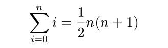
Proof:
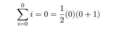
First, we have to verify the base case
Then we assume
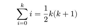
as our inductive hypothesis, and argue as follows
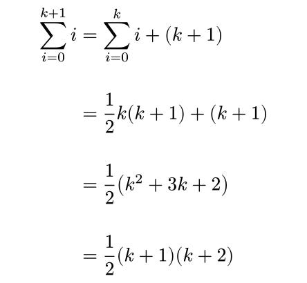
Thus by the principle of induction, the proposition holds for all natural numbers.
2. Inductive Types
Most axiomatisations of the natural numbers include the principle of induction or some statement equivalent to it. One common formulation states that if a subset of the natural numbers contains zero and is closed under the successor function, then that subset is the whole set of naturals. In this formulation, our proof above showed precisely that the set
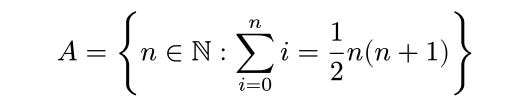
contains 0, and that it is closed under taking successors, and therefore that it is equal to ℕ. The underlying idea here is that a natural number is either 0 or the successor of some other natural number and that there are no other possibilities. In this sense, you can build ℕ starting with only 0 and using only the successor function.
One way to bake this idea into the definition is to define the naturals in the form of an inductive type. We define the naturals as everything you can get by repeatedly applying the constructor (the successor function) to the constant 0.
We can define other inductive types like this, for example lists of integers. We start with a constant “nil”, which represents the empty list; Our constructor is then a function denoted :: which takes a natural number n and a list L, and outputs the list n::L, where n is appended to the start of L. For example 6::[1,2,3] = [6,1,2,3]. More explicitly:
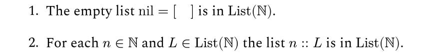
The nature of this definition allows us to perform inductive proofs here too.
Proposition 2.1:
Every list is finite.
Proof:
Firstly nil is finite. Then, if L is finite, n::L is finite. Therefore by induction, all lists are finite.
3. Coinductive Types
As proposition 2.1 shows, the list type isn’t capable of handling infinite content. You can’t build infinite things from finite things in finitely many steps. If we want to express infinite data-types then we’ll need a new kind of definition.
Let’s do an example, and consider infinite lists, which from now on we’ll refer to as streams. As before, we can append something to the front of a stream such as 6::[1,4,9,16,25, … ] = [6,1,4,9,16,25, … ]. But this time this doesn’t give us a way to build all of the streams in the same way as with the lists. We don’t have anywhere to start from!
However, this time we can also consider the other direction. Given any stream S we can break S into two parts; we can extract the first element called the head of S, or we can discard the first element and just take the rest which we call the tail of S which will be a new stream. In notation this is

If you completely specify the head and tail of S, then you completely specify S. For example, if

then S is the stream [7,7,7,7, … ] and if

then S₀ = [0,1,2,3,4,5, … ].
Just as every inductive type comes with an induction principle, every coinductive type comes with a coinduction principle — which we’ll construct in the next few parts.
4. Fixed Points
To figure out what coinduction principles look like, we should start by describing induction principles in more generality.
An inductive type is built from a set of constants and a set of constructors. For ℕ, this was 0 and the constructor was n ↦ n+1. We formulated the principle of induction to say that if a set contained 0, and was closed under the successor function, then that set contained all of ℕ. We can express this principle in the following statement:

The idea here is that if A is closed under the successor function, then for every a in A, a+1 is in A, which precisely means that the set of all of the a+1s is a subset of A. The same reasoning applies to 0.
For lists, if we make the identification n::L = (n, L) then we can phrase the induction principle there as

Notably, in both cases, if we replace A with ℕ or List(ℕ), the ⊆ relation becomes an equality. To generalise these we consider monotone set-valued functions. These map sets to sets (not values of sets!) satisfying the following relationship:

You can verify that both of the above examples are monotone. Then we say that a set X is “F-closed” if and only if

And that X is “F-consistent” if and only if

Then define μF as the intersection of all F-closed sets.
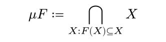
Proposition 4.1:
μF is a fixed point for F.
Proof:
Firstly we have:

which since F is monotone implies

which from the definition of μF as an intersection implies

which together with the first statement implies

In this sense, μF is the least fixed point of F. And we can use this fact to formulate induction in a highly general way:
Theorem 4.2 (Principle of Induction):
If F is a monotone set-valued function and X is a set in the domain of F, then

The proof is immediate from the above work.
Notably, the argument for proposition 4.2 also works to characterise a greatest fixed point of F. Define νF to be the union of F-consistent sets, i.e.
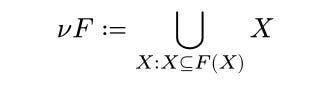
and then since this is the greatest fixed point of F we get:
Theorem 4.3 (Principle of Coinduction):
If F is a monotone set-valued function and X is a set in the domain of F, then

Let’s do a simple example to illustrate. The set of streams Stream(ℕ) satisfies

and further more, we have that

and so for any set X, it follows by coinduction that

5. Applications of Coinduction
As it may initially appear, coinduction doesn’t look that powerful. With induction, if you want to prove a property of μF, you can write down an F-closed set which has that property, and the result follows immediately for μF. In contrast, with νF, it looks like all you can do is prove that something is a subset of νF.
It turns out, however, that by carefully choosing F we can still prove very powerful results. For this, we will study the lexicographic ordering on the set of streams.
The lexicographic ordering is defined as follows: we say that σ ≤ τ if and only if

Intuitively, if the first elements are different you stop there. If they’re not, then you look at the next element of the stream and keep going until you find a difference. Since a relation between streams is a subset of Stream(ℕ)², we can identify ≤ with the subset

Then if we define the function

It is easy to show that ≤ is νT.
Proposition 5.1:
The lexicographic ordering on streams is transitive. i.e. if ≤ is the lexicographic order then

Proof:
Consider the set

and suppose we have streams σ, ρ, and τ such that σ ≤ ρ ≤ τ. By definition of ≤, we have
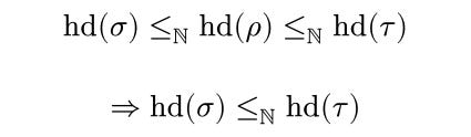
Now suppose that hd(σ) = hd(τ). We get that

by the definition of ≤. This immediately implies that (tl(σ), tl(τ)) is an element of R. In turn, this means that R is T-consistent which means we can apply coinduciton! We conclude:

or in other words that

which is exactly what we were trying to show.
Unless you’re doing specific kinds of functional programming, you’re not very likely to need coinductive types or to use coinduction as a proof technique — most mathematicians don’t know about it or use it, because in a lot of situations there are other ways to prove these results, even if coinduction would be simpler or quicker.
That’s not really the point, however. The point is that we described an existing technique in a new way, and used that to develop interesting generalisations and ideas that we wouldn’t have thought about otherwise. A lot of the most powerful and insightful mathematics was discovered by this kind of process.
For those who know category theory, some good further reading would be to look at the concepts of initial algebras and final co-algebras — which encode the work we’ve been doing here in a categorical concept, and make the duality at play even more explicit.
Thanks for reading :)
References and Further reading:
https://www.cs.cornell.edu/~kozen/Papers/Structural.pdf
This is the main paper this article is based on, though I rephrased or reformulated quite a few things, and didn’t touch on the more in depth and advanced mathematical logic.
https://ncatlab.org/nlab/show/algebra+for+an+endofunctor
This is a good place to start the further reading on the category stuff.
https://www.andrew.cmu.edu/user/avigad/Talks/qpf.pdf
More relevant further reading on inductive and coinductive types and their categorical semantics — a little experience with the lean proof language is also helpful.